Challenge 4 - Building a Demand Forecast

Introduction

BigQuery ML can be used to build and deploy demand forecasting models using the ARIMA_PLUS algorithm. In this section, you use BigQuery ML to build a model to forecast the demand for products in store.

Description

Prepare your training data

Here you will use parts of the replicated data as training data to your model.

The training data describes for each product (product_name), how many units were sold (total_sold) per hour (hourly_timestamp).

Using the BigQuery console, run the following SQL to create and save the training data to a new training_data table:

 CREATE OR REPLACE TABLE `retail.training_data`
 AS
     SELECT
         TIMESTAMP_TRUNC(time_of_sale, HOUR) as hourly_timestamp, product_name, 
         SUM(quantity) AS total_sold
     FROM `retail.ORDERS`
     GROUP BY hourly_timestamp, product_name
     HAVING hourly_timestamp 
     BETWEEN TIMESTAMP_TRUNC('2021-11-22', HOUR) AND TIMESTAMP_TRUNC('2021-11-28', HOUR)
 ORDER BY hourly_timestamp

Run the following SQL to verify the training_data table:

 SELECT * FROM `retail.training_data` LIMIT 10;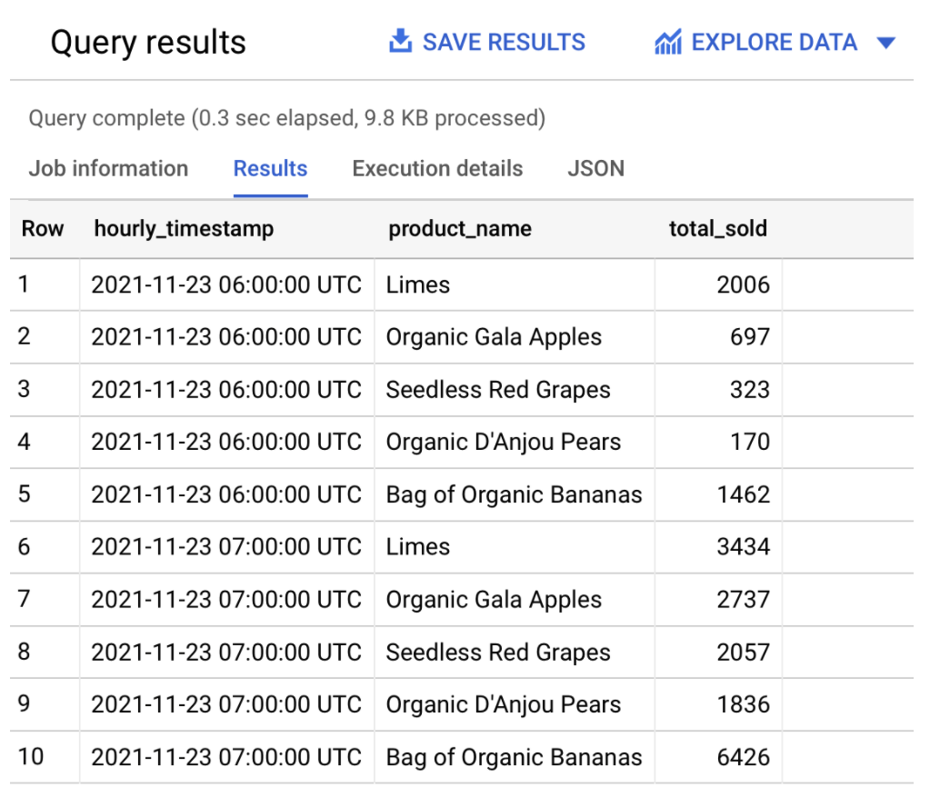

Training Query Results

Forecast Demand

Still In BigQuery, execute the following SQL to create a time-series model that uses the ARIMA_PLUS algorithm:

Options to use for model named: retail.arima_plus_model:
```
 MODEL_TYPE='ARIMA_PLUS',
 TIME_SERIES_TIMESTAMP_COL='hourly_timestamp',
 TIME_SERIES_DATA_COL='total_sold',
 TIME_SERIES_ID_COL='product_name'
```
SQL to use:
```
 QUERY hourly_timestamp, product_name AND total_sold FROM OBJECT retail.training_data
```
NOTE: Look at the Creating ARIMA_PLUS Model documentation in the Learning Resources section below.
Run the following SQL to forecast the demand for organic bananas over the next 30 days:

NOTE: The ML.FORECAST function is used to forecast the expected demand over a horizon of n hours.
```
 SELECT * FROM ML.FORECAST(MODEL retail.arima_plus_model, STRUCT(720 AS horizon))
```
The output should be similar to:

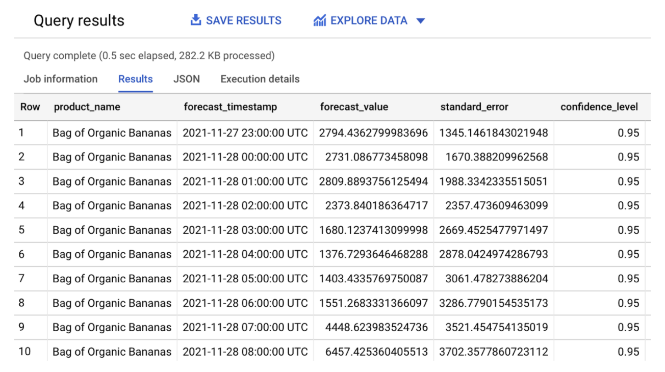
Because the training data is hourly, the horizon value will use the same unit of time when forecasting (hours). A horizon value of 720 hours will return forecast results over the next 30 days.

NOTE: Since this is a small sample dataset, further investigation into the accuracy of the model is out of scope for this tutorial.

Create a view for easier visualization

In BigQuery, run the following SQL query to create a view, joining the actual and forecasted sales for a given product:

 CREATE OR REPLACE VIEW retail.orders_forecast AS (
 SELECT
 timestamp,
 product_name,
 SUM(forecast_value) AS forecast,
 SUM(actual_value) AS actual
 FROM
 (
 SELECT
     TIMESTAMP_TRUNC(TIME_OF_SALE, HOUR) AS timestamp,
     product_name,
     SUM(QUANTITY) as actual_value,
     NULL AS forecast_value
     FROM retail.ORDERS
     GROUP BY timestamp, product_name
 UNION ALL
 SELECT
     forecast_timestamp AS timestamp,
     product_name,
     NULL AS actual_value,
     forecast_value,
         FROM ML.FORECAST(MODEL retail.arima_plus_model,
             STRUCT(720 AS horizon))
     ORDER BY timestamp
 )
 GROUP BY timestamp, product_name
 ORDER BY timestamp
 )    

NOTE: This view lets Looker query the relevant data when you explore the actual and forecasted data.

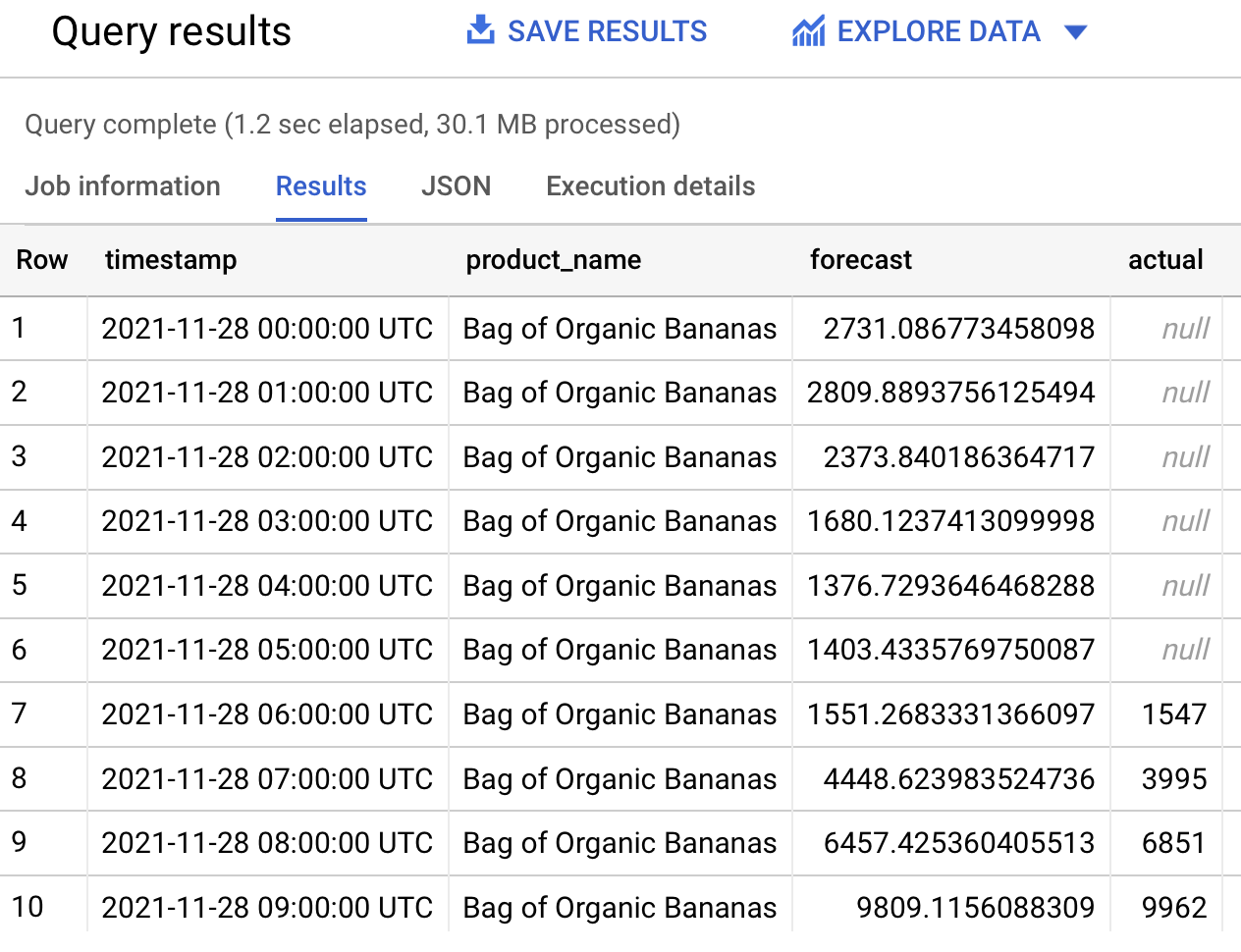
Still in BigQuery, run the following SQL to validate the view:
```
 SELECT * FROM retail.orders_forecast
 WHERE PRODUCT_NAME='Bag of Organic Bananas'
 AND TIMESTAMP_TRUNC(timestamp, HOUR) BETWEEN TIMESTAMP_TRUNC('2021-11-28', HOUR) AND TIMESTAMP_TRUNC('2021-11-30', HOUR)
 LIMIT 100;
```
You see an output that is similar to the following:

As an alternative to BigQuery views, you can also use Looker’s built-in derived tables capabilities. These include built-in derived tables and SQL-based derived tables. For more information, see Derived Tables in Looker.

Success Criteria

Table retail.training_data created
ARIMA model retail.arima_plus_model created
View retail.orders_forecast created